Fair federated learning under heterogeneity

Keep the average.
Protect the clients. FedPCD: Priority-Constrained Federated Aggregation

A federated aggregation rule that follows the FedAvg direction and bends it only as much as needed to give every client a minimum of progress. It has one tolerance τ, keeps a short server-side memory of recently seen clients, and returns the FedAvg direction unchanged whenever no client falls short.

Yousef Irshaid★,1 Dara Varam★,1,2 Mohamed I. AlHajri1
1 American University of Sharjah 2 Senseable City Lab, MIT ★ Equal contribution

Preprint · under review

TL;DR

FedAvg trains one model for many clients by averaging their updates. When clients hold very different data, that average can make little, no, or even negative progress for some of them. Existing fairness-aware methods reweight clients, correct conflicting updates, or search for a common descent direction, and in doing so they often change the global direction or treat every client as a symmetric peer. FedPCD keeps the FedAvg direction as the primary objective and turns every client into a minimum-progress constraint. The server takes the direction closest to the average that still gives each client a τ-fraction of progress, and it remembers recently seen clients so that partial participation does not leave them unprotected. When the average already serves everyone, the direction is exactly FedAvg's.

18 / 18 settings with the highest global accuracy 17 / 18 with the highest worst-10% client accuracy 71.9% vs 48.1% for FedAvg CIFAR-10, α = 0.01, 5% participation 10–44% of the rounds to reach FedAvg's final accuracy

Video

The whole idea, animated.

A ten-minute tour: why the average can leave clients behind, how FedPCD's projection and its client history work, what the theory guarantees, and the results on CIFAR-10, CIFAR-100 and Fashion-MNIST.

Narration voice generated with ElevenLabs.

The mechanism, interactively

FedAvg averages. FedPCD checks every client.

Three clients send updates that pull in different directions, and their normalized average g̃0 is the FedAvg direction. Each client asks for a minimum of progress, g̃i⊤d̃ ≥ τ‖g̃i‖², which admits a half-space of directions. FedPCD projects the average onto the shaded region where every client is satisfied. Drag the client arrows and slide τ to see when the average has to bend, and by how much.

In the figure (click a layer to hide it)

At τ = 0, FedPCD only asks that no client gets worse, to first order. A larger τ tightens every constraint, and the update bends further toward the clients that need it.

Client directions

Unit client directions in two dimensions, with equal weights. The experiments use τ between 0.005 and 0.1. It is larger here so that the geometry is easy to see.

An interactive version of the gradient-space panel of Figure 2 in the paper, in the same colors. It opens on the paper's example: clients at 10°, 45° and 155° with τ = 0.25. Only client 3's constraint is active there, so the update is the average plus μ3⋆ = 0.36 of client 3's direction, and the other two clients still get more than their minimum.

The idea

The average sets the course. Clients decide when it bends.

FedPCD is a federated adaptation of Priority-Constrained Descent (PCD), a method for problems in which one objective matters more than the others. Here the FedAvg update takes the primary role, and each client's own update defines a secondary constraint.

Each participating client returns its model displacement Δi,t after K local steps, as in FedAvg. The server divides it by the local learning rate to obtain a pseudo-gradient, and aggregates these with the FedAvg weights:

\[ g_{i,t} \;=\; \frac{\Delta_{i,t}}{\eta_\ell} \;=\; \frac{\theta_t-\theta_{i,t}^{(K)}}{\eta_\ell}, \qquad \bar g_t \;=\; \sum_{i\in\mathcal{S}_t} \bar p_{i,t}\, g_{i,t} \]

The aggregate and every client direction are then normalized:

\[ \tilde g_{0,t} \;=\; \frac{\bar g_t}{\lVert\bar g_t\rVert+\varepsilon}, \qquad \tilde g_{i,t} \;=\; \frac{g_{i,t}}{\lVert g_{i,t}\rVert+\varepsilon} \]

The update is the direction closest to the normalized average that still makes a τ-fraction of progress along every client's direction:

\[ \tilde d_t^\star \;=\; \arg\min_{\tilde d}\; \frac{1}{2}\left\lVert \tilde d-\tilde g_{0,t}\right\rVert^2 \quad \mathrm{s.t.} \quad \tilde g_{i,t}^{\top}\tilde d \;\geq\; \tau \lVert \tilde g_{i,t}\rVert^2, \qquad i\in\mathcal{S}_t \]

Each constraint is a half-space of acceptable directions. This small convex quadratic program is therefore the Euclidean projection of the FedAvg direction onto their intersection, and its solution is unique. Its optimality conditions give it one revealing form:

\[ \tilde d_t^\star \;=\; \tilde g_{0,t} \;+\; \sum_{i\in\mathcal{A}} \mu_i^\star\, \tilde g_{i,t}, \qquad \mu_i^\star \geq 0 \]

The average keeps a coefficient of one. A client enters only through a non-negative multiplier, and that multiplier is zero unless the client's constraint is active. FedPCD does not replace the global update with a reweighted or symmetric multi-objective direction. It retains the average as the primary direction and applies the minimal correction that the clients require.

Because the program works with normalized directions, the server rescales the solution to the length of the aggregate before taking the step:

\[ d_t \;=\; \frac{\lVert \bar g_t\rVert}{\lVert \tilde d_t^\star\rVert}\,\tilde d_t^\star, \qquad \theta_{t+1} \;=\; \theta_t-\eta_g\, d_t \]

When nothing needs fixing. If the average already satisfies every constraint, then d̃⋆ = g̃0, and the rescaling gives dt = ḡt. FedPCD introduces no directional correction in that round.
One round of FedPCD

Algorithm 1 in the paper. On the clients, it is a FedAvg round.

  1. ClientsThe server samples St and broadcasts θt. Each sampled client trains locally for K steps and sends back Δi,t.
  2. ServerForm the pseudo-gradients gi,t = Δi,t / ηℓ and their weighted aggregate ḡt.
  3. ServerDrop cache entries older than H rounds. The ones that remain, hi,t, become constraints too.
  4. ServerNormalize every direction and solve the program for d̃⋆.
  5. ServerRescale to ‖ḡt‖, update θt+1 = θt − ηgdt, and store the participants' current pseudo-gradients in the cache.
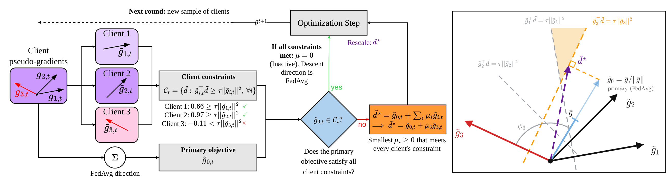
FedPCD system diagram: client pseudo-gradients feed the client constraints and the primary FedAvg direction. If the primary direction satisfies every constraint the step is FedAvg; otherwise the smallest correction is added. A gradient-space panel shows the projection.
The system diagram of the paper, for three participating clients at round t. Left: the steps that produce the final direction. Right: the same example in gradient space. The half-space of each client defines the feasible region, and the projection shows the minimum distortion needed to satisfy every client.

Partial participation

A short memory for the clients who are away.

In practice only 5% or 10% of clients join each round, so each round's program sees only a handful of them. A client with unusual data can go unseen for many rounds, and while it is away nothing protects it.

FedPCD gives the server a history window of H rounds. It keeps the most recent pseudo-gradient of every client that took part within the window, and each cached direction adds one more constraint, h̃i,t⊤d̃ ≥ τ‖h̃i,t‖². A client that returns overwrites its entry, and an entry older than H rounds is removed. The primary direction ḡt is still computed only from the clients of the current round. History changes who is protected, not what the average is.

Under independent uniform participation at rate ρ, the expected number of distinct clients represented once the window has filled is

\[ N\left(1-(1-\rho)^{H+1}\right) \]

With N = 100 clients, ρ = 0.1 and H = 10, that is about 69 clients in every program instead of 10.

0 of 100 clients constrain the update in round 0

Participation ρ

A simulation of the cache alone: 100 clients, sampled uniformly without replacement each round, as in the experiments. Set H = 0 to see what the program holds without history.

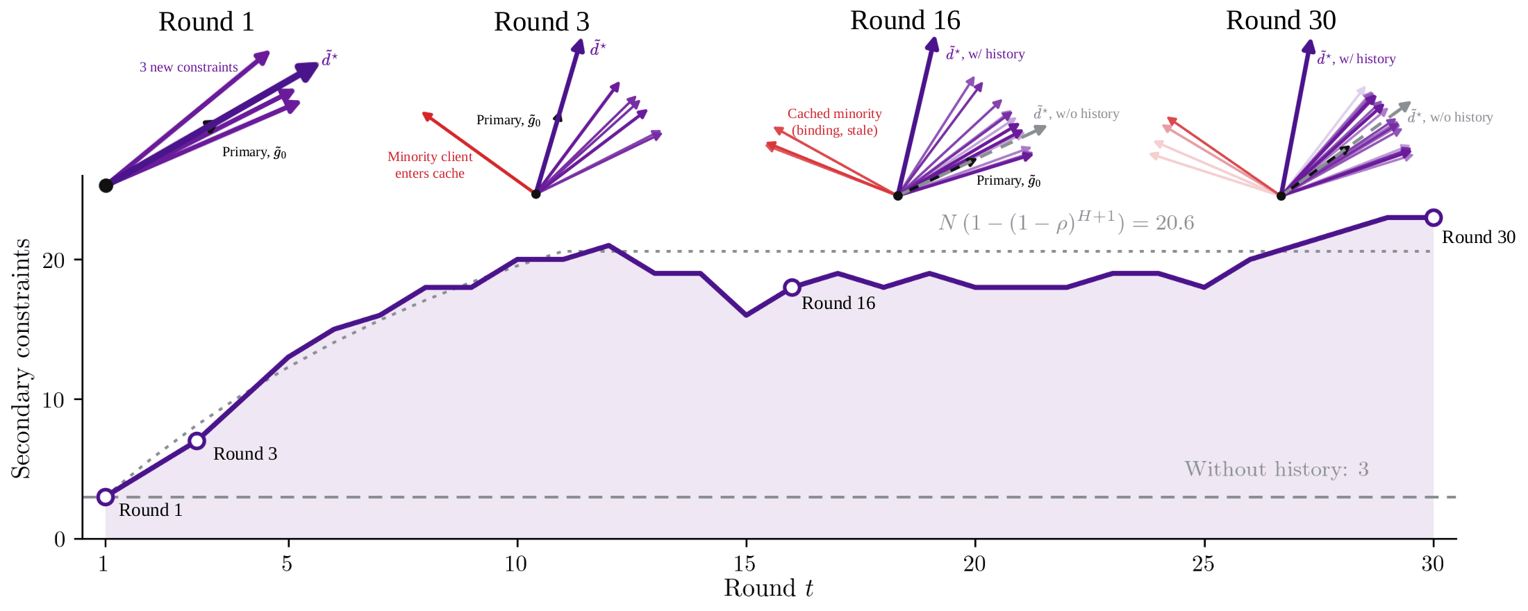
Demonstration of history: the constrained program at rounds 1, 3, 16 and 30, and the number of secondary constraints per round rising from 3 toward about 20.
The paper's synthetic demonstration, with N = 30 clients, 10% participation, H = 10 and τ = 0.1. Top: the program at four rounds. Paler arrows are older cache entries, and red arrows are minority clients that do not satisfy the constraint. Bottom: the number of secondary constraints per round. Without history the program never holds more than three. In round 16 no minority client is sampled, but a cached one still constrains the update, and d̃⋆ with and without history point in different directions.

The window is a trade-off. A longer one represents more clients, and it also keeps older directions.

Guarantees

What the constrained update guarantees.

01

A minimum of progress for every client

Whenever the program is feasible, its solution satisfies g̃i,t⊤d̃⋆ ≥ τ‖g̃i,t‖² for every client of the round and for every cached client. With τ > 0, the update is positively aligned with each of them by construction.

02

Unchanged when no client falls short

If the normalized average already meets every constraint, the projection is the identity and d̃⋆ = g̃0. After rescaling, dt = ḡt: the round keeps the conventional federated direction, with no correction.

03

The smallest correction, at FedAvg's step length

Otherwise the solution is the unique closest admissible direction to the average, and only active constraints contribute to it. The result is rescaled to ‖ḡt‖, so the program changes the direction of the update and not its magnitude.

04

An O(1/T) rate

With full participation, deterministic local steps, no history, L-smooth client objectives and a uniform alignment margin γ, the round-averaged squared norm of the global gradient falls as O(1/T) with constant learning rates, including for K > 1 local steps (Theorem 4.1).

05

Every client stationary, not just their average

The same rate holds for the clients' own gradients. Under the same conditions every accumulation point is composite multi-stationary: each client is stationary on its own. That is stronger than Pareto stationarity, where nonzero client gradients may simply cancel (Corollary 4.2).

∎

Full proofs in the paper

The alignment and local-drift lemmas, the descent argument behind the rate, and a careful account of what the client-progress and stationarity statements do and do not cover.

See the appendix →

Theorem 4.1, for a server step 0 < ηg ≤ γeff / (LK(1+r)). Here r measures the drift of K local steps and γeff = γ(1−r) − r is the alignment margin that remains after it. The margin γ describes the geometry of the constrained direction and is not a hyperparameter.

\[ \frac{1}{T}\sum_{t=0}^{T-1}\left\lVert\nabla F(\theta_t)\right\rVert^2 \;\leq\; \frac{2\left[F(\theta_0)-F_\star\right]}{\eta_g\,\gamma_{\mathrm{eff}}\,\gamma\,K(1-r)\,T} \;=\; \mathcal{O}(1/T) \]

Results

A higher average, a stronger tail, fewer rounds.

CIFAR-10, CIFAR-100 and Fashion-MNIST with 100 clients, at 5% and 10% participation and three levels of heterogeneity. That makes 18 settings, each averaged over five seeds, against ten baselines: FedAvg, AFL, q-FFL, Ditto, FedMGDA+, FedFV, FedLF, FedHEAL, FedPW and CRAFT.

18 / 18
settings in which FedPCD has the highest global accuracy ā. On CIFAR-100 it leads the strongest competitor, CRAFT, by 1.7 to 5.6 points.
17 / 18
settings in which it also has the highest worst-10% client accuracy W10%. The exception is Fashion-MNIST at 10% participation and α = 0.01, where FedLF reaches 65.73% against 63.22%.
10–44%
of the communication rounds are enough to reach FedAvg's final accuracy. FedPCD also reaches the strongest baseline's final accuracy earlier in 16 of the 18 settings.
Figures at heterogeneity A smaller α means more heterogeneous clients. The text beside each figure describes α = 0.01, the hardest setting. All figures fix τ = 0.02 and H = 10.
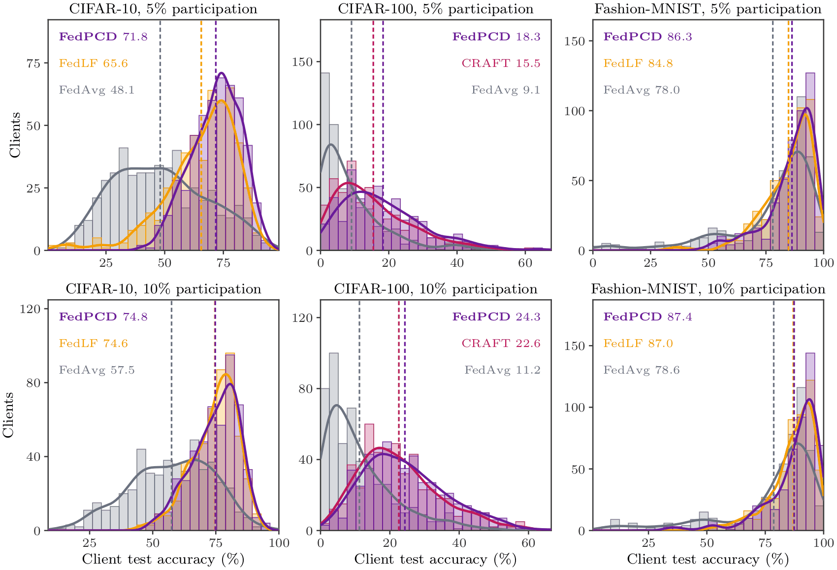
Histograms of per-client test accuracy for FedPCD, FedAvg and the strongest baseline, on three datasets and two participation rates.
Per-client test accuracy at α = 0.01, pooled over five seeds, for FedPCD, FedAvg and the strongest baseline of each setting. Dashed lines mark the means.

The gains reach the clients who need them

On CIFAR-10 at 5% participation, FedPCD reaches 71.90% global accuracy, against 65.59% for the strongest baseline, FedLF, and 48.09% for FedAvg. Its worst 10% of clients reach 52.88%, more than 14 points above FedLF's.

Compared with FedAvg, the whole distribution of client accuracies moves to the right and its lower tail thins out. Compared with the strongest baseline, more of the clients sit near the top.

Numbers in the text are those of the paper's Table 1, at FedPCD's best τ. The figures fix τ = 0.02, so their labels differ slightly.

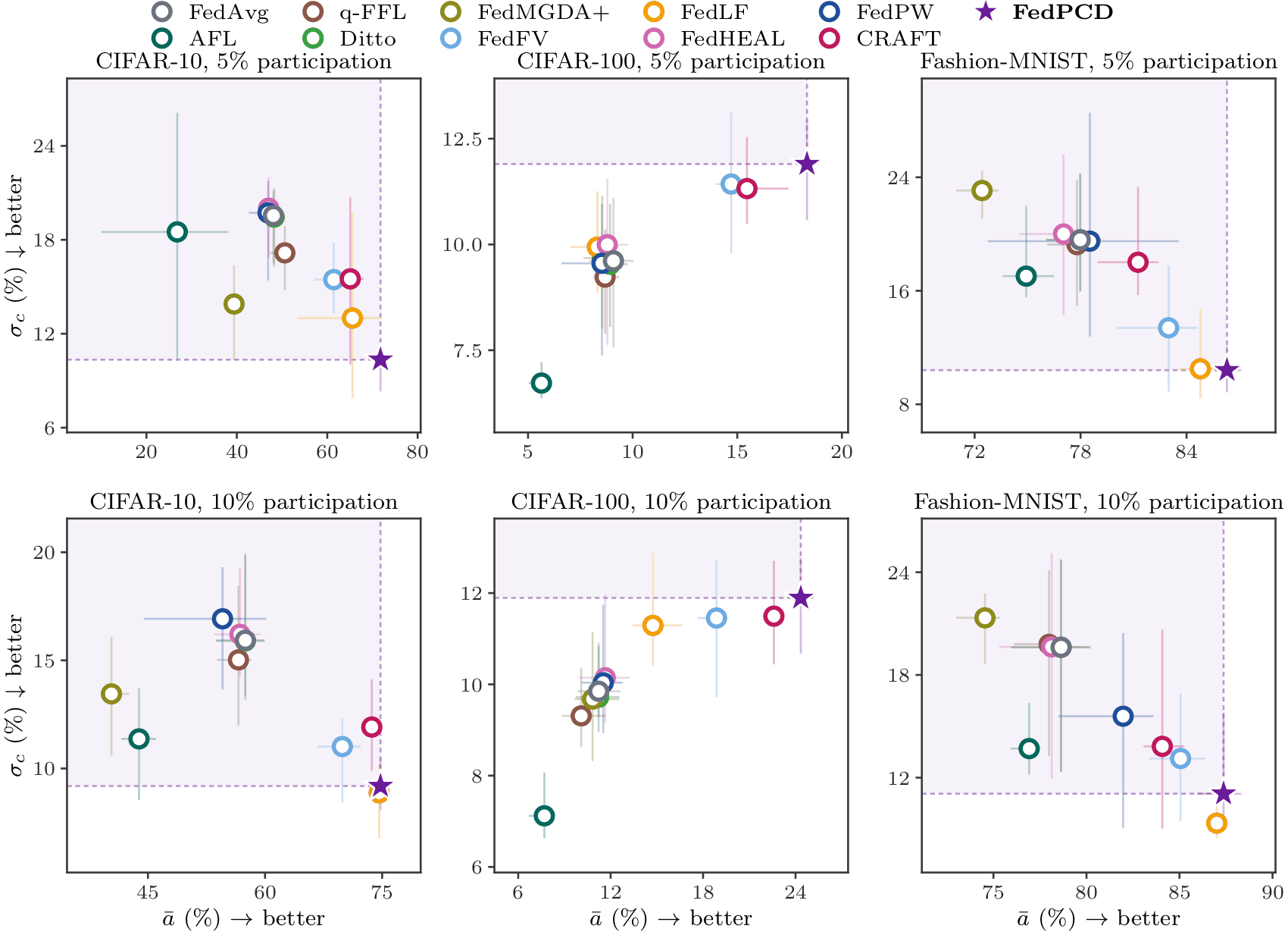
Global accuracy against the spread of client accuracies for all eleven methods; FedPCD sits at or near the bottom-right corner.
Global accuracy ā against client spread σc at α = 0.01. The arrows on the axes point toward better, so the bottom-right corner is best. Crosses show the range over the five seeds.

Even, without holding everyone down

Spread alone can mislead, because a method can look even by keeping every client low. On CIFAR-100, AFL has the lowest σc in all six settings, at global accuracies between 5.64% and 14.55%.

Plotted against accuracy, FedPCD is at least as accurate and at least as even as all ten baselines on CIFAR-10 and Fashion-MNIST at 5% participation, and as at least nine of the ten at 10%.

On CIFAR-100 its spread is higher than the baselines', because σc grows with the accuracy it is measured around. Jain's fairness index does not, and it ranks FedPCD first in all six CIFAR-100 settings.

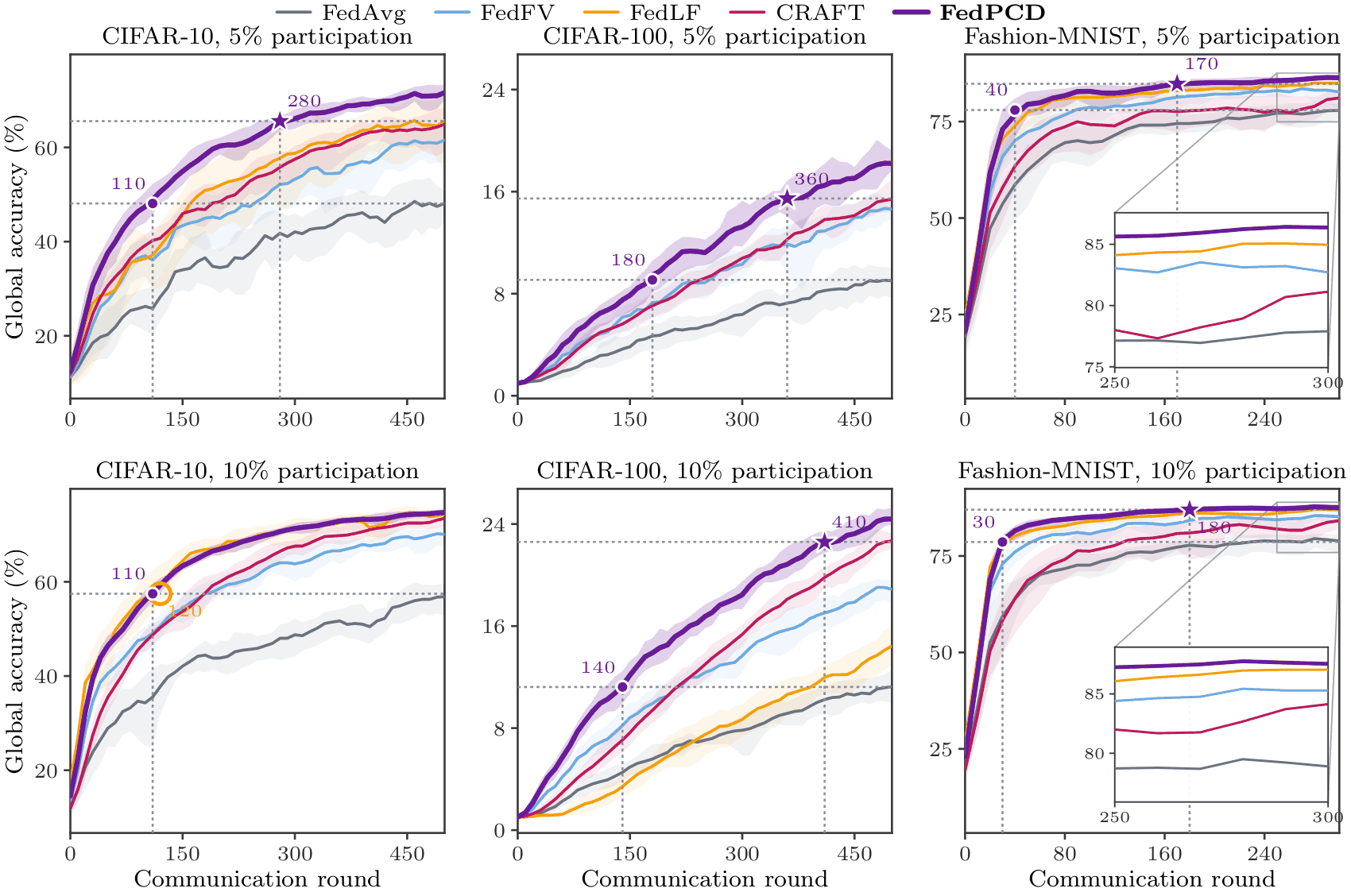
Global accuracy against communication round for FedPCD, FedAvg and the three strongest baselines; FedPCD reaches FedAvg's final accuracy much earlier.
Global accuracy against communication rounds at α = 0.01, for FedAvg, FedPCD and the three strongest baselines. Dots mark where FedPCD reaches FedAvg's final accuracy, and stars where it reaches the strongest baseline's. Where it does not, a hollow ring marks where that baseline reaches FedAvg's final accuracy.

The same accuracy in fewer rounds

On CIFAR-10, FedPCD reaches FedAvg's final accuracy by round 110 of 500, about 4.5× fewer rounds. At 5% participation it reaches the final accuracy of the strongest baseline by round 280.

On CIFAR-100 it matches FedAvg's final accuracy by rounds 180 and 140, at 5% and 10% participation. On Fashion-MNIST it needs 40 and 30 of the 300 rounds.

What matters

History does most of the work. Every part helps.

Take the history away and FedPCD falls from 74.84% to 59.26% on CIFAR-10, close to FedAvg's 57.47%. The other components cost less to remove, and each of them still costs something.

Component ablation

CIFAR-10, 10% participation, α = 0.01, five seeds

VariantGlobal accuracyā (%) ↑W10% ↑
FedPCD74.8458.03
with τ = 074.3157.55
without normalization72.9954.44
without the primary direction70.7546.86
without history59.2629.65
FedAvg57.4729.93

From the paper's component ablation. Variants with history use τ = 0.01, the best value for this setting in Table 1. The history-free variant uses its own best tested value, τ = 0.1.

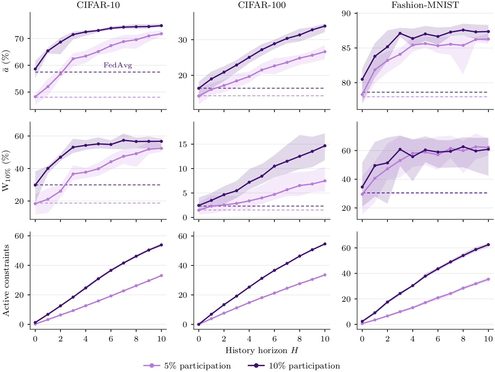
Global accuracy, worst-10% accuracy and the number of active constraints as the history window grows from 0 to 10 rounds, on three datasets.
The history window sweep at τ = 0.02 and α = 0.01. Top: global accuracy, with FedAvg dashed. Middle: worst-10% accuracy. Bottom: the number of active constraints. On CIFAR-10 at 5% participation, global accuracy climbs from below 50% without history to above 70% with a ten-round window. The largest gains come from the first few rounds of memory, and the returns diminish after that even though the number of constraints keeps growing.

Scope

What FedPCD assumes, and what it does not claim.

  • The convergence theorem covers full participation, deterministic local steps and no history (H = 0). Stochastic gradients, partial participation and cached directions are outside it. The experiments use all three, so the theorem describes an idealized version of what is run.
  • The rate also assumes that the program stays feasible and that its solution keeps a uniform alignment margin γ > 0 with every nonzero client pseudo-gradient, at every round. This is a real restriction on the client directions and not a consequence of smoothness. Two exactly opposite client directions, for instance, cannot both make positive progress.
  • The composite multi-stationarity conclusion is conditional on that geometry. Arbitrary heterogeneous client objectives need not share a stationary point.
  • Client protection means first-order directional progress. It is not a guarantee that every client's loss decreases at every round, and it is not a guarantee about client accuracy.
  • FedPCD does not lead on every metric. On Fashion-MNIST at 10% participation and α = 0.01, FedLF has the better worst-10% accuracy and the lower spread. On CIFAR-100, FedPCD's σc is higher than the baselines'.
  • τ is one fixed value for all clients and rounds, and the best value shifts with heterogeneity. The headline counts use the best of six tested values in each setting, as the paper's text does. With a single τ = 0.02 throughout, Table 1 still gives FedPCD the highest global accuracy in all 18 settings, and the highest worst-10% accuracy in 15.
  • The server has to see each client's pseudo-gradient individually and keep it for H rounds. That limits the use of FedPCD with secure aggregation, and motivates privacy-compatible variants.
  • The evaluation uses 100 clients, one local epoch and three image-classification benchmarks. Behavior under many local steps, where client drift degrades the pseudo-gradient directions, is not established.

Citation

Cite FedPCD

@misc{irshaid2026fedpcd,
  title  = {{FedPCD}: Priority-Constrained Federated Aggregation},
  author = {Irshaid, Yousef and Varam, Dara and AlHajri, Mohamed I.},
  year   = {2026},
  note   = {Preprint, under review},
  url    = {https://daravaram.github.io/FedPCD/}
}

FedPCD builds on Priority-Constrained Descent (TMLR 2026). This entry will be updated when the preprint is on arXiv.

Copied to clipboard