Priority-Constrained Descent (PCD)

TL;DR

Most training pipelines mix several losses, but one is usually the real deliverable (task accuracy) while the rest only constrain it (sparsity, low-rank, fidelity). Symmetric multi-objective methods average all gradients as equal peers and can stall before the primary has converged. PCD anchors to the primary gradient and admits only the minimal distortion needed to keep every secondary making guaranteed progress — one bounded knob τ, no weight search, and a fixed point that is reached only when every objective is individually stationary.

1 dial, not a weight sweep 94.0% acc @ 90% pruning DenseNet-121 / CIFAR-10 70.9% acc @ 90% pruning ResNet-34 / CIFAR-100 Can't get trapped in conflict equilibria

The mechanism, interactively

Symmetric methods average. PCD prioritizes.

Every gradient-based multi-objective method takes the primary gradient g₁ and the secondary gradient g₂ and composes a single update d^★. Drag the gradient handles to change the geometry, and slide τ to set how hard the secondary pushes. Watch how the symmetric methods treat the two objectives as interchangeable, while PCD stays pinned to the primary and projects onto the shaded feasible region.

Tolerance τ0.20

τ = 0 reverts to the symmetric (Pareto) endpoint; larger τ forces stronger secondary progress.

Gradient configuration

Conflict ∠(g₁,g₂)105° Secondary strength ‖g₂‖0.70

Drag g₂ in the figure, or use these. When ‖g₂‖ = 1 the symmetric methods (WS, MGDA, CAGrad) collapse onto a single line — only PCD stays distinct.

Methods (click to toggle)

FAMO and AuxiNash are history- / bargaining-based; their update can't be drawn from a single gradient snapshot, so they're shown only in the results below.

An interactive remake of Figure 3 in the paper. The four symmetric methods are label-symmetric — swapping g₁ and g₂ leaves their update unchanged. PCD is the only one whose primary coefficient is structurally pinned to one.

The idea

Anchor to the primary. Distort the minimum amount.

Let g̃₁, …, g̃_K be the scale-normalized gradients of the primary and secondary objectives. PCD takes the direction closest to the primary gradient that still guarantees a τ-fraction of progress on every secondary:

\[ \mathbf{d}^\star \;=\; \operatorname*{arg\,min}_{\mathbf{d}\in\mathbb{R}^n}\; \bigl\lVert \mathbf{d}-\tilde{\mathbf{g}}_1 \bigr\rVert^2 \quad\text{s.t.}\quad \tilde{\mathbf{g}}_j^{\!\top}\mathbf{d} \;\ge\; \tau\,\bigl\lVert\tilde{\mathbf{g}}_j\bigr\rVert^2 \quad \forall\, j \ge 2 \]

This small convex quadratic program is exactly the Euclidean projection of the primary gradient onto the polyhedron of admissible directions. Its KKT solution has one revealing form:

\[ \mathbf{d}^\star \;=\; \tilde{\mathbf{g}}_1 \;+\; \sum_{j\ge 2}\mu_j^\star\,\tilde{\mathbf{g}}_j, \qquad \mu_j^\star \ge 0 \]

The primary's coefficient is pinned to one; each secondary enters only through a non-negative multiplier that is zero unless its constraint is active. The "anchor" and the "corrections" are built into the construction — not recovered from it. That is the structural break from symmetric methods, which mix g₁ and g₂ as peers and cannot tell the deliverable from its constraints.

For K = 2 the update is fully closed-form — add exactly the component along g̃₂ needed to meet the constraint at equality, and no more. K = 3 is closed-form via Cramer's rule; larger K uses an active-set solver whose O(K²n) cost is dominated by the K backpropagations.

\[ \mathbf{d}^\star = \begin{cases} \tilde{\mathbf{g}}_1, & \tilde{\mathbf{g}}_2^{\!\top}\tilde{\mathbf{g}}_1 \ge \tau\lVert\tilde{\mathbf{g}}_2\rVert^2,\\[6pt] \tilde{\mathbf{g}}_1 + \Bigl(\tau - \dfrac{\tilde{\mathbf{g}}_2^{\!\top}\tilde{\mathbf{g}}_1}{\lVert\tilde{\mathbf{g}}_2\rVert^2}\Bigr)\,\tilde{\mathbf{g}}_2, & \text{otherwise.} \end{cases} \]

Scale invariance. Gradients are normalized by an EMA of their squared norm, so ‖g̃_j‖ ≈ 1 in steady state. That makes τ interpretable on [0,1] regardless of loss magnitudes, and the update invariant to per-objective rescaling — a property weighted sum provably lacks.

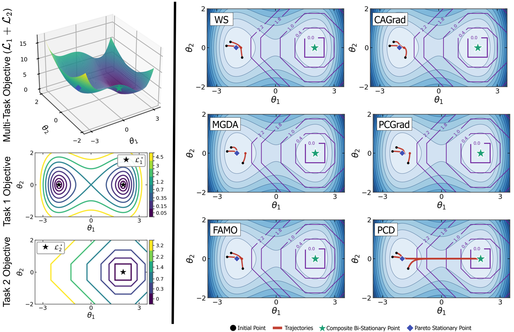
Six optimizers on a double-well multi-task landscape; PCD alone crosses the saddle to the joint minimum. — On a 2D problem where ℒ₁ has two minima — only one of which also minimizes ℒ₂ — every symmetric baseline (WS, CAGrad, MGDA, PCGrad, FAMO) stalls at a conflict equilibrium where ℒ₂ is still non-zero. PCD alone crosses the saddle to the point where ∇ℒ₁ = ∇ℒ₂ = 0.

What PCD guarantees

Five properties, proven.

01

Per-step secondary progress

With τ > 0 and a feasible QP, every step satisfies g̃_j^⊤d^★ ≥ τ‖g̃_j‖² — a tolerance-controlled descent on each non-stationary secondary. Stronger than PCGrad (no per-objective guarantee), MGDA (only an aggregate), and weighted sum (only the scalarized loss).

02

Falls back to clean SGD

When the primary direction already gives enough progress on every secondary, the projection is the identity and d^★ = g̃₁ exactly. The secondaries never perturb the primary when they don't have to.

03

Scale invariance

EMA normalization makes the update invariant under per-objective rescaling ℒ_i → c_iℒ_i, so τ keeps a consistent, scale-free meaning even when raw loss magnitudes differ by orders of magnitude.

04

A strictly stronger endpoint

d^★ = 0 if and only if every objective is individually stationary — composite multi-stationarity. It is strictly stronger than Pareto stationarity and rules out the gradient-cancellation conflict equilibria where symmetric methods halt.

05

One bounded dial

Sweeping τ ∈ [0,1] varies the feasible set monotonically and traces a continuous trade-off curve between the Pareto endpoint (τ=0) and the CMS endpoint. No weight ratios, conflict coefficients, or per-loss schedules to search.

∎

Full proofs in the paper

Farkas feasibility, the projection / KKT theorem, scale invariance, and the CMS and τ=0 endpoint characterizations — with a clickable theory map.

See the appendix →

Results

Near-unpruned accuracy where baselines collapse.

70.9%

accuracy at 90% structured sparsity on ResNet-34 / CIFAR-100 (73.3% unpruned). Strongest baseline (AuxiNash): 44.4%.

89.2%

accuracy at 99% parameter reduction on DenseNet-121 / CIFAR-10 — a 43.2× FLOPs and 97.2× model-size cut.

2.3–3.4×

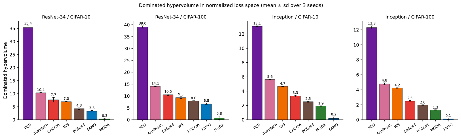
the dominated hypervolume of the strongest baseline in the three-objective setting, in every configuration.

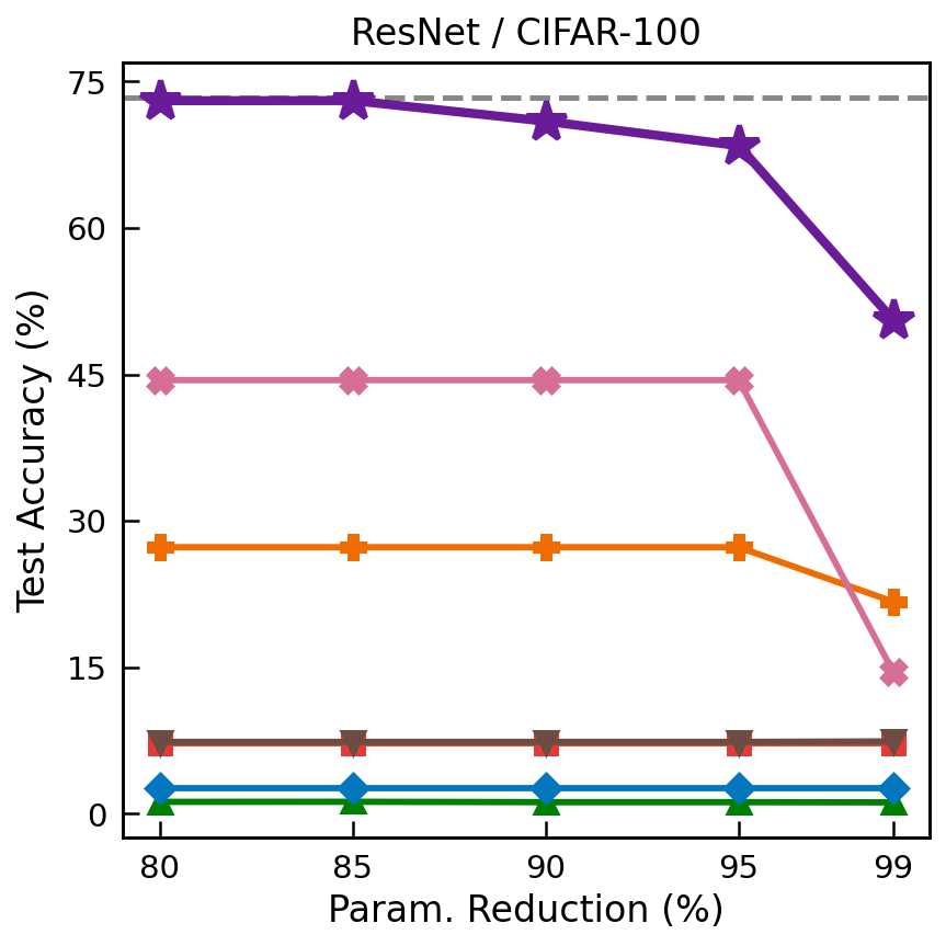
Accuracy vs parameter reduction; PCD stays far above all baselines.

One method dominates the pruning frontier

Across four architectures (DenseNet-121, ResNet-34, Inception, MobileNetV2) on CIFAR-10 and CIFAR-100 — eight configurations — PCD's purple curve sits above every multi-objective baseline at every compression target. Under a structural sparsity penalty the symmetric direction methods (MGDA, PCGrad, CAGrad, FAMO) collapse toward random accuracy; PCD holds the line.

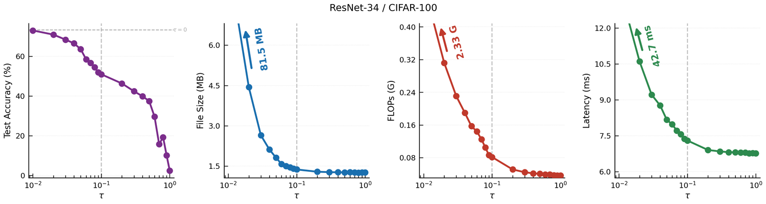
Accuracy, file size, FLOPs and latency as a function of τ.

One dial, the whole frontier

Sweeping a single τ trades 81.5 MB of size, 2.33 G FLOPs and 42.7 ms of latency against accuracy on ResNet-34 / CIFAR-100. The curve is smooth and monotone — most of the benefit arrives within τ ∈ (0, 0.1] — so a practitioner dials to a resource budget instead of searching weight ratios.

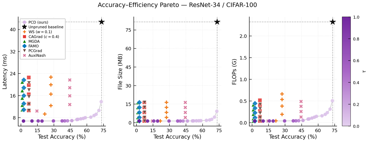
Pareto frontiers of accuracy vs latency, size and FLOPs.

The swept front dominates baselines

On every resource axis — latency, file size, FLOPs — PCD's τ-swept curve lies above each baseline's best operating point. The same single knob that controls compression traces the entire accuracy–efficiency Pareto front.

Where it applies

Anywhere a loss is one deliverable plus structural conditions.

Structured pruning & compression

Pair the task loss with a group-lasso, ℓ₁, or nuclear-norm penalty; τ becomes a single compression dial that traces a smooth accuracy–efficiency curve.

Quantization-aware training

Keep the task loss primary and a fidelity term penalizing drift from quantized parameters as the secondary, anchoring the model against discrete-value drift without hand-tuned weights.

Federated & personalized learning

Hold local fitness as the deliverable against communication-budget or personalization terms, with τ modulating how hard those constraints push.

Structured generative modeling

For flow matching and VAEs, keep generative fidelity primary while structural regularizers act as constraints rather than competing peers.

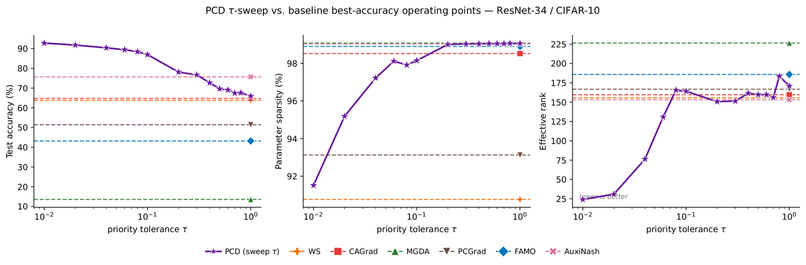
Beyond two objectives — a K = 3 hierarchy (task loss + ℓ₁ sparsity + nuclear-norm low-rank):

τ-sweep on a three-objective hierarchy versus baseline operating points. — A single τ-sweep beats every baseline on accuracy and effective rank at once; at τ = 0.02, ResNet-34 / CIFAR-100 holds **71.0%** accuracy at effective rank **24.5**, versus AuxiNash's 48.7% at rank 184.8.

Dominated hypervolume per configuration; PCD largest everywhere. — Dominated hypervolume in the normalized three-objective space: PCD covers the most of the joint trade-off surface in every configuration.

Scope

What PCD assumes — and what it doesn't claim.

Secondaries are assumed proper, convex, lower-semicontinuous with accessible subgradients (ℓ₁, group lasso, nuclear norm, total variation, hinge all qualify). Non-convex secondaries fall outside the guarantees, though the algorithm still runs.
Guarantees are local and directional — they attach to the normalized direction d^★ and its idealized first-order step, not to a stochastic global-convergence claim.
The CMS endpoint is meaningful only when a jointly stationary point exists (the regularizer-style hierarchy). On genuine trade-offs with no common stationary point, τ > 0 has no fixed point.
For K > 2 the QP can be infeasible if secondaries are mutually incompatible — but in high dimensions this is a measure-zero event (0 of 1785 synthetic feasibility checks were infeasible).
Each step needs K backpropagations for the gradients; the K×K QP itself is negligible — the same O(K²n) order as MGDA.

Citation

Cite PCD

@article{varam2026pcd,
  title         = {Not All Objectives Are Born Equal: Priority-Constrained
                   Descent for Hierarchical Multi-Objective Optimization},
  author        = {Varam, Dara and AlHajri, Mohamed I.},
  journal       = {arXiv preprint arXiv:2606.29521},
  year          = {2026},
  eprint        = {2606.29521},
  archivePrefix = {arXiv},
  primaryClass  = {cs.LG},
  url           = {https://arxiv.org/abs/2606.29521}
}